Data Science in Python for Climate Data Analysis
gdfa.ugr.es/python
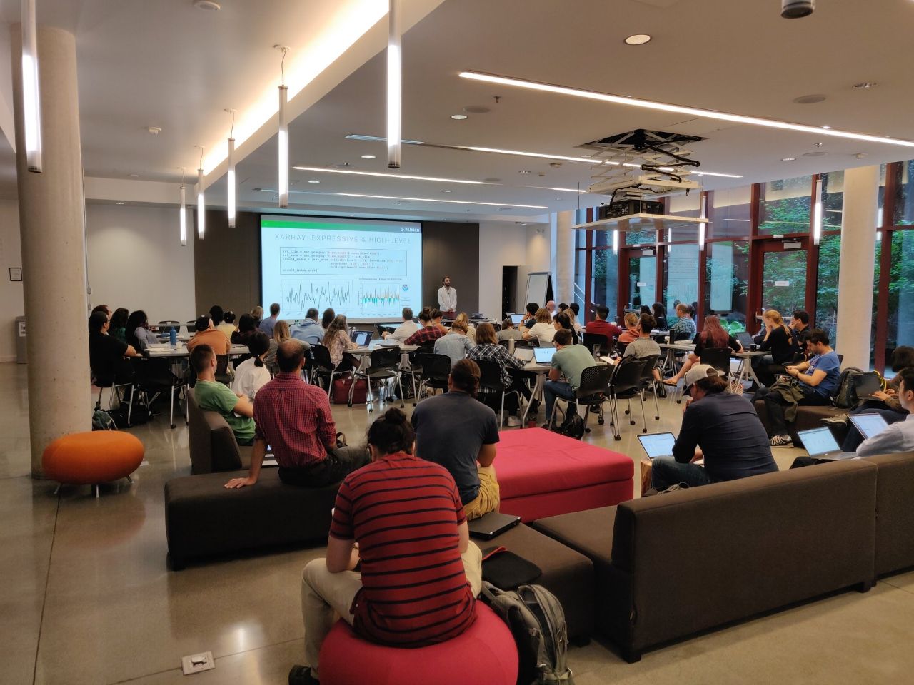
Oceanhackweek, University of Washington (Aug 26-30, 2019)
- Download-analyze model: data analysts first download the desired dataset from a remote server to local workstations or cluster infrastructure, in order to perform the desired analysis
Problem: the size and variety of datasets have increased exponentially and new data science methodologies have appeared
CF Conventions
- The Climate and Forecast (CF) metadata conventions are conventions for the description of Earth sciences data, intended to promote the processing and sharing of data files. The CF conventions were introduced in 2003, after several years of development by a collaboration that included staff from U.S. and European climate and weather laboratories
- In December 2008 the trio of standards, netCDF+CF+OPeNDAP, was adopted by IOOS as a recommended standard for the representation and transport of gridded data. The CF conventions are being considered by the NASA Standards Process Group (SPG) and others as more broadly applicable standards
- CF originated as a standard for data written in netCDF, but its structure is general and it has been adapted for use with other data formats
OPeNDAP
- An attempt focused on enhancing the retrieval of remote, structured data through a Web-based architecture
- Client may construct DAP constraint expressions to retrieve specific content (i.e., subsets)
- OPeNDAP servers offer various types of responses, including XML, JSON, HTML, ASCII or NetCDF
- ECMWF: Copernicus (ERA5), ESGF: NASA, NOAA... (CMIP5, CORDEX)
In [1]:
from IPython.display import IFrame
IFrame("http://opendap.puertos.es/thredds/catalog.html", width=1200, height=600)
Out[1]:
xarray

- xarray is inspired by and borrows heavily from pandas
- It is particularly tailored to working with netCDF files
- It integrates tightly with dask for parallel computin
In [2]:
%matplotlib inline
In [3]:
import warnings
warnings.simplefilter("ignore")
In [4]:
%ls data/*.nc
In [5]:
import xarray as xr
ds = xr.open_dataset("data/total_precipitation.nc")
In [6]:
ds
Out[6]:
In [7]:
ds = xr.open_mfdataset("data/*.nc", combine="by_coords") # , parallel=True
In [8]:
ds
Out[8]:
In [9]:
ds_noaa = xr.open_dataset(
"http://www.esrl.noaa.gov/psd/thredds/dodsC/Datasets/noaa.ersst.v5/sst.mnmean.nc"
)
In [10]:
ds_noaa
Out[10]:
lazy loading of:
- on-disk datasets or
- remote
In [11]:
main_var = "swh"
aux_var = "tp"
In [12]:
ds[main_var]
Out[12]:
In [13]:
time_ini = "2000-01-01"
time_end = "2002-12-31"
longitude = -22
latitude = 16
In [14]:
ds[main_var].sel(time=slice(time_ini, time_end)).plot()
Out[14]:

The purpose of visualization is insight, not pictures
― Ben Shneiderman


In [15]:
import hvplot.xarray
In [16]:
ds[main_var].sel(time=slice(time_ini, time_end)).hvplot()
Out[16]:
In [17]:
ds[main_var].sel(longitude=longitude, latitude=latitude, method="nearest").hvplot()
Out[17]:
In [18]:
ds[main_var].sel(longitude=longitude, latitude=latitude, method="nearest").groupby(
"time.month"
).mean().hvplot()
Out[18]:
In [19]:
ds[main_var].sel(time=slice(time_ini, time_end)).sel(
longitude=longitude, latitude=latitude, method="nearest"
).hvplot()
Out[19]:
In [20]:
import cartopy.crs as ccrs
import numpy as np
import matplotlib.pyplot as plt
proj = ccrs.PlateCarree()
In [21]:
figsize = (10, 5)
zoom = 1
lon_min = ds.coords["longitude"].min()
lon_max = ds.coords["longitude"].max()
lat_min = ds.coords["latitude"].min()
lat_max = ds.coords["latitude"].max()
extent = [
lon_min - zoom * 0.5,
lon_max + zoom * 0.5,
lat_min - zoom * 0.5,
lat_max + zoom * 0.5,
]
resolution = "50m"
In [22]:
def default_map(axes=None, global_map=False, background=True):
if axes is None:
fig, ax = plt.subplots(figsize=figsize, subplot_kw={"projection": proj})
else:
ax = axes
if global_map:
ax.set_global()
else:
ax.set_extent(extent)
ax.coastlines(resolution=resolution)
if background:
ax.stock_img()
return ax
In [23]:
ax = default_map(global_map=True)
plt.scatter(
ds.coords["longitude"][0],
ds.coords["latitude"][0],
c="navy",
s=100,
marker="o",
edgecolors="white",
alpha=0.9,
)
plt.show()

In [24]:
ax = default_map(background=False)
lons, lats = np.meshgrid(ds.coords["longitude"], ds.coords["latitude"])
plt.scatter(lons, lats, c="blue", s=1)
plt.show()

In [25]:
import geoviews.feature as gf
ds[main_var].isel(time=0).hvplot(
"longitude", "latitude", crs=proj, cmap="viridis", width=500, height=500
) * gf.coastline.options(scale=resolution, line_width=2)
Out[25]:
In [26]:
df = ds.sel(longitude=longitude, latitude=latitude, method="nearest").to_dataframe()[
main_var
]
df
Out[26]:
In [27]:
df.to_csv("data/swh.csv", header=True)
In [28]:
df.to_csv("data/swh.zip", header=True) # compression="zip"
In [29]:
%ls -lh data/swh*
In [30]:
%ls -lh data/SIMAR*
In [31]:
import pandas as pd
df_file = pd.read_csv("data/swh.zip", index_col="time", parse_dates=True)
In [32]:
df_file
Out[32]:
In [33]:
df_simar = pd.read_csv(
"data/SIMAR_1052046",
delim_whitespace=True,
skiprows=80,
parse_dates=[[0, 1, 2, 3]],
index_col=0,
header=0,
na_values=-99.9,
)
In [34]:
df_simar.to_csv("data/SIMAR_1052046.zip", header=True)
In [35]:
import hvplot.pandas
df_file.hvplot()
Out[35]:
Third-party netCDF packages:
- NCO: package of command line operators that manipulates generic netCDF data and supports some CF conventions
- CDO: a collection of command-line operators to manipulate and analyze climate and numerical weather prediction data; includes support for netCDF-3, netCDF-4 and GRIB1, GRIB2, and other formats
- NCL: interpreted language for scientific data analysis and visualization
Main Tutorials (https://oceanhackweek.github.io/curriculum_2019.html)
- Access and Clean-up Ocean Observation Data
- Data Visualization Part I: Basics and Geospatial Visualization
- Advanced Data Visualization
- Cloud Computing 101
- Handle "Big" Larger-than-memory Data
- Pangeo
- Machine Learning
- Git, GitHub and Project Collaboration
- Reproducible Research
Project: Co-Locators
This project aims to provide a way to Co-locate oceanographic data by establishing constraints. The tools developed allow users to provide geospacial bounds in a temporal range to get an aggregated response of all available data.