Outline
- Why learn programming? Why learn Python?
- Some samples
- Python highlights
- Python for science, where to begin?
- Python language
- Scientific libraries
Why learn programming? Why learn Python?


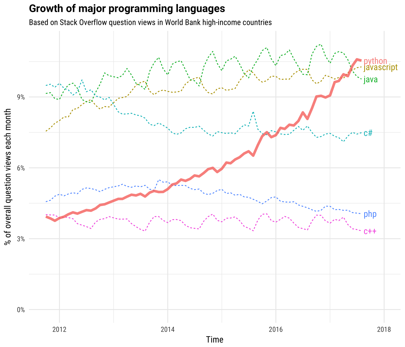
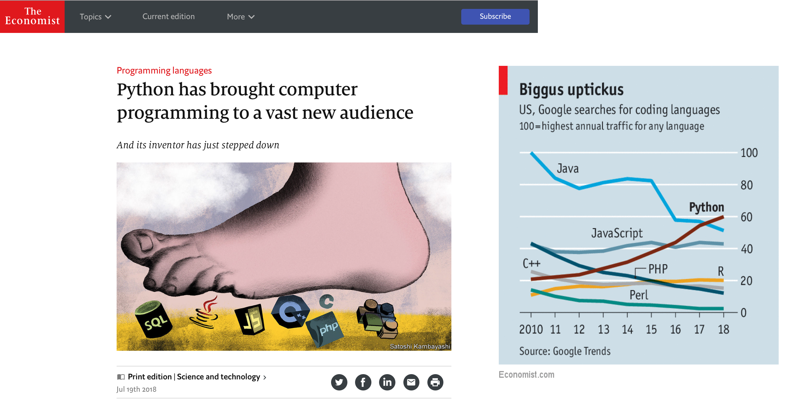

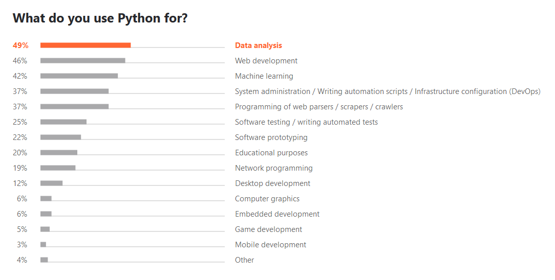
Where is Python mostly used?
- YouTube
- DropBox
- Netflix
- ...
Some samples
Study cases:
Researchers solve problems that are highly specific to their field of expertise. These problems cannot be solved by the straightforward application of off-the-shelf software, so researchers develop tools that are bound to their exact needs.
Almost every office worker uses a laptop as a daily tool. Computers are such a huge productivity booster because they support a large market of programs designed for these workers. But these applications don't automate every conceivable task. Coding can save workers time of effort.
External file required:
import pandas as pd

# required to show plots inside Jupyter
%matplotlib inline

df = pd.read_csv("GlobalTemperatures.csv", parse_dates=["dt"], index_col="dt")
madrid = df[df.City == "Madrid"]

madrid["AverageTemperature"].plot()
<matplotlib.axes._subplots.AxesSubplot at 0x118be0b70>
import hvplot.pandas

madrid["AverageTemperature"].hvplot()
madrid["AverageTemperature"].groupby(madrid.index.year).mean().plot()
<matplotlib.axes._subplots.AxesSubplot at 0x10a8e3e48>
madrid["AverageTemperature"].groupby(madrid.index.year).mean().hvplot()
import geoviews as gv
import geoviews.feature as gf

cities = (
    df.groupby("City")
    .max()
    .rename(columns={"AverageTemperature": "MaximumTemperature"})
)
dataset = gv.Dataset(cities)
points = dataset.to(
    gv.Points,
    ["Longitude", "Latitude"],
    ["MaximumTemperature", "AverageTemperatureUncertainty", "Country"],
)
gv.extension("matplotlib")  # required to show static plots

gf.coastline.opts(fig_size=300) * points
gv.extension("bokeh")  # required to show insteractive plots

gf.coastline.opts(width=600, height=350) * points.opts(
    tools=["hover"], size=(gv.dim("MaximumTemperature") - 10) * 0.5
)
# http://wxmaps.org/fcst.php

from IPython.display import IFrame
IFrame("http://wxmaps.org/fcst.php", width=1200, height=600)
import requests

base_url = "http://wxmaps.org/pix/"
name = "aus7.48hr.png"

r = requests.get(base_url + name)
with open(f"output/{name}", "wb") as f:
    f.write(r.content)
regions = {
    "North America": "avnmr",
    "North America (NAM, 12-Hourly)": "nam",
    "South America": "sa",
    "Europe": "euro",
    "Africa": "af",
    "Australia & New Zealand": "aus",
    "East Asia": "ea",
    "Central Asia": "casia",
    "India": "india",
    "Northern Hemisphere": "hemi",
    "Southern Hemisphere": "shemi",
    "Tropics": "trop",
}
products = {
    "Heights": "1",
    "SLP": "2",
    "Precipitation": "3",
    "Temperature": "4",
    "Streamlines": "5",
    "Precipitable water": "6",
    "Cloud cover": "7",
}
forecasts = {
    "Analysis": "00",
    "Day 1": "24",
    "Day 2": "48",
    "Day 3": "72",
    "Day 4": "96",
    "Day 5": "120",
    "Day 6": "144",
}
rg = regions["Australia & New Zealand"]
pr = products["SLP"]
fr = forecasts["Day 1"]

name = f"{rg}{pr}.{fr}hr.png"
print(name)
aus2.24hr.png
r = requests.get(base_url + name)
print("Downloading " + name + "...")
with open(f"output/{name}", "wb") as f:
    f.write(r.content)
Downloading aus2.24hr.png...
import time

rg = regions["Europe"]
pr = products["SLP"]

# limit the number of downloads for a demo
n = 0
limit = 3

for forecast in forecasts.values():
    name = f"{rg}{pr}.{forecast}hr.png"
    output_name = f"output/{name}"

    if n < limit:
        r = requests.get(base_url + name)
        print("Downloading " + name + "...")

        with open(output_name, "wb") as f:
            f.write(r.content)

        n += 1
        time.sleep(1)
Downloading euro2.00hr.png...
Downloading euro2.24hr.png...
Downloading euro2.48hr.png...
rg = regions["Europe"]

# limit the number of downloads for a demo
n = 0
limit = 3

for forecast in forecasts.values():
    for product in products.values():
        name = f"{rg}{product}.{forecast}hr.png"
        output_name = f"output/{name}"

        if n < limit:
            r = requests.get(base_url + name)
            print("Downloading " + name + "...")

            with open(output_name, "wb") as f:
                f.write(r.content)

            n += 1
            time.sleep(1)
Downloading euro1.00hr.png...
Downloading euro2.00hr.png...
Downloading euro3.00hr.png...
# limit the number of downloads for a demo
n = 0
limit = 3

for forecast in forecasts.values():
    for product in products.values():
        for region in regions.values():
            name = f"{region}{product}.{forecast}hr.png"
            output_name = f"output/{name}"

            if n < limit:
                r = requests.get(base_url + name)
                print("Downloading " + name + "...")

                with open(output_name, "wb") as f:
                    f.write(r.content)

                n += 1
                time.sleep(1)
Downloading avnmr1.00hr.png...
Downloading nam1.00hr.png...
Downloading sa1.00hr.png...
Python highlights
What is Python?
Python is a modern, general-purpose, object-oriented, high-level programming language.
General characteristics of Python:
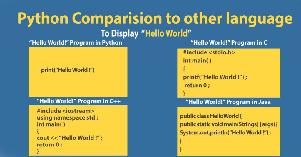
- clean and simple language: Easy-to-read and intuitive code, easy-to-learn minimalistic syntax, maintainability scales well with size of projects.
- expressive language: Fewer lines of code, fewer bugs, easier to maintain.
Technical details:
- dynamically typed: No need to define the type of variables, function arguments or return types.
- automatic memory management: No need to explicitly allocate and deallocate memory for variables and data arrays. No memory leak bugs.
- interpreted: No need to compile the code. The Python interpreter reads and executes the python code directly.
Advantages:
- The main advantage is ease of programming, minimizing the time required to develop, debug and maintain the code.
- Well designed language that encourage many good programming practices:
- Modular and object-oriented programming, good system for packaging and re-use of code. This often results in more transparent, maintainable and bug-free code.
- Documentation tightly integrated with the code.
- A large standard library, and a large collection of add-on packages.
- Packaging of programs into standard executables, that work on computers without Python installed.
Disadvantages:
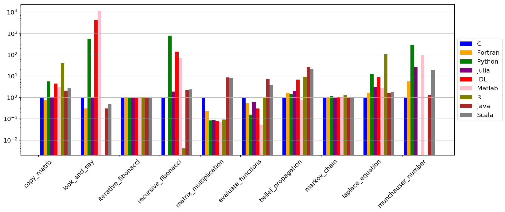
- Since Python is an interpreted and dynamically typed programming language, the execution of python code can be slow compared to compiled statically typed programming languages, such as C and Fortran.
- Somewhat decentralized, with different environment, packages and documentation spread out at different places. Can make it harder to get started.
What makes python suitable for scientific computing?
| Nature 518, 125-126 (05 February 2015) doi:10.1038/518125a |
Nature 563, 145-146 (30 October 2018) doi:10.1038/d41586-018-07196-1 |
 |
 |
Python for science, where to begin?
Scientific-oriented Python Distributions
Provide a Python interpreter with commonly used scientific libraries in science like NumPy, SciPy, Pandas, matplotlib, etc. already installed. In the past, it was usually painful to build some of these packages. Also, include development environments with advanced editing, debugging and introspection features.
-
- Most widely adopted
- Cross-platform

# https://www.anaconda.com/distribution/#download-section

IFrame("https://www.anaconda.com/distribution/#download-section", width=1200, height=600)
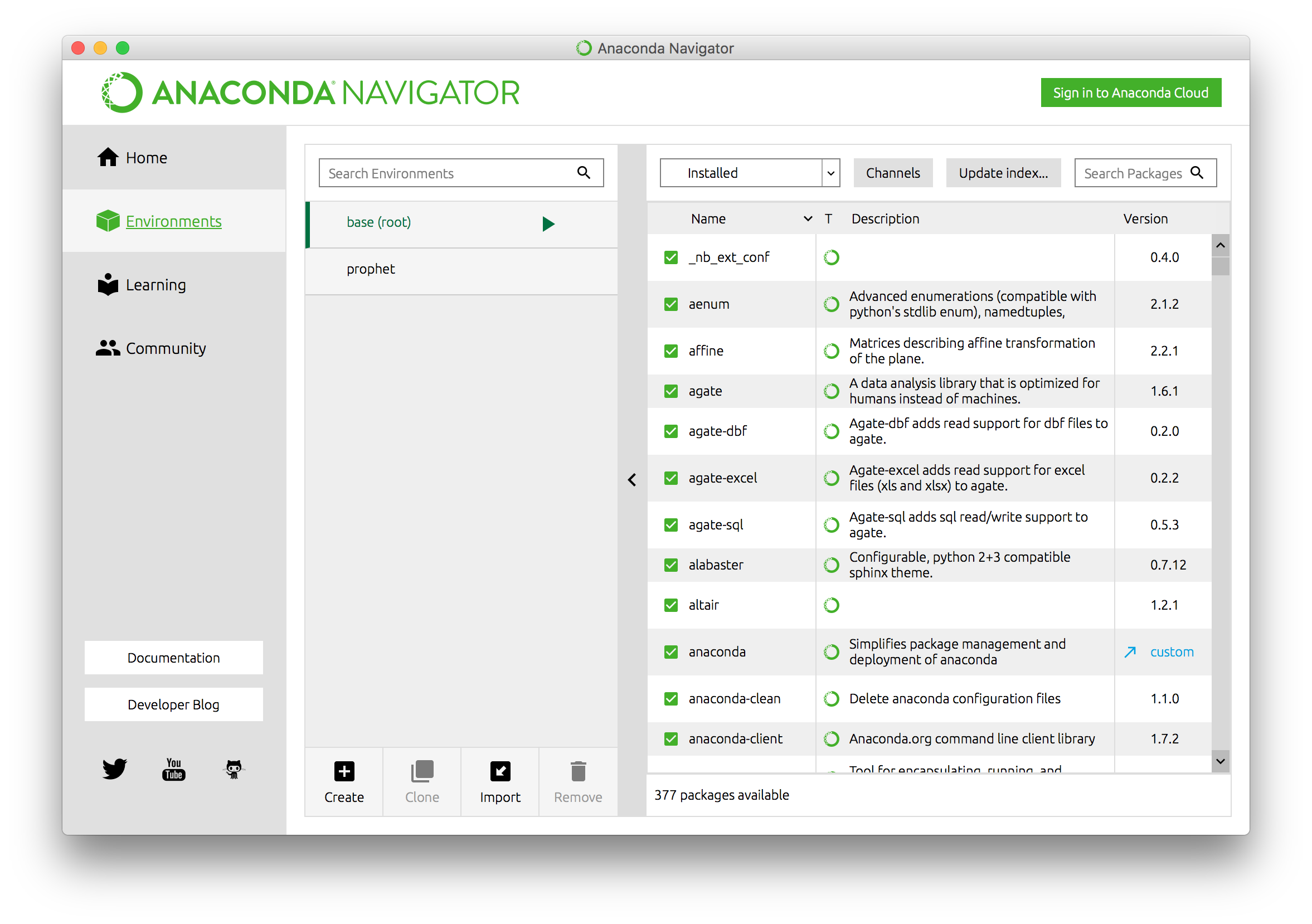
Anaconda navigator

Anaconda navigator: installing new packages
Spyder

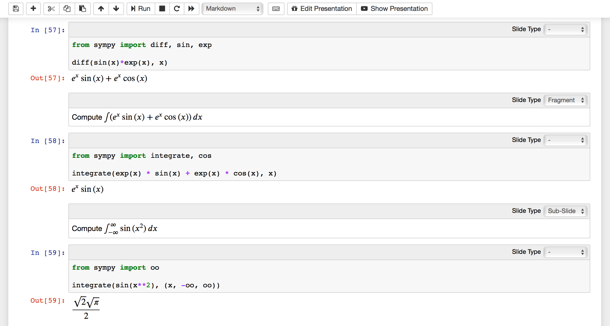
Jupyter notebooks
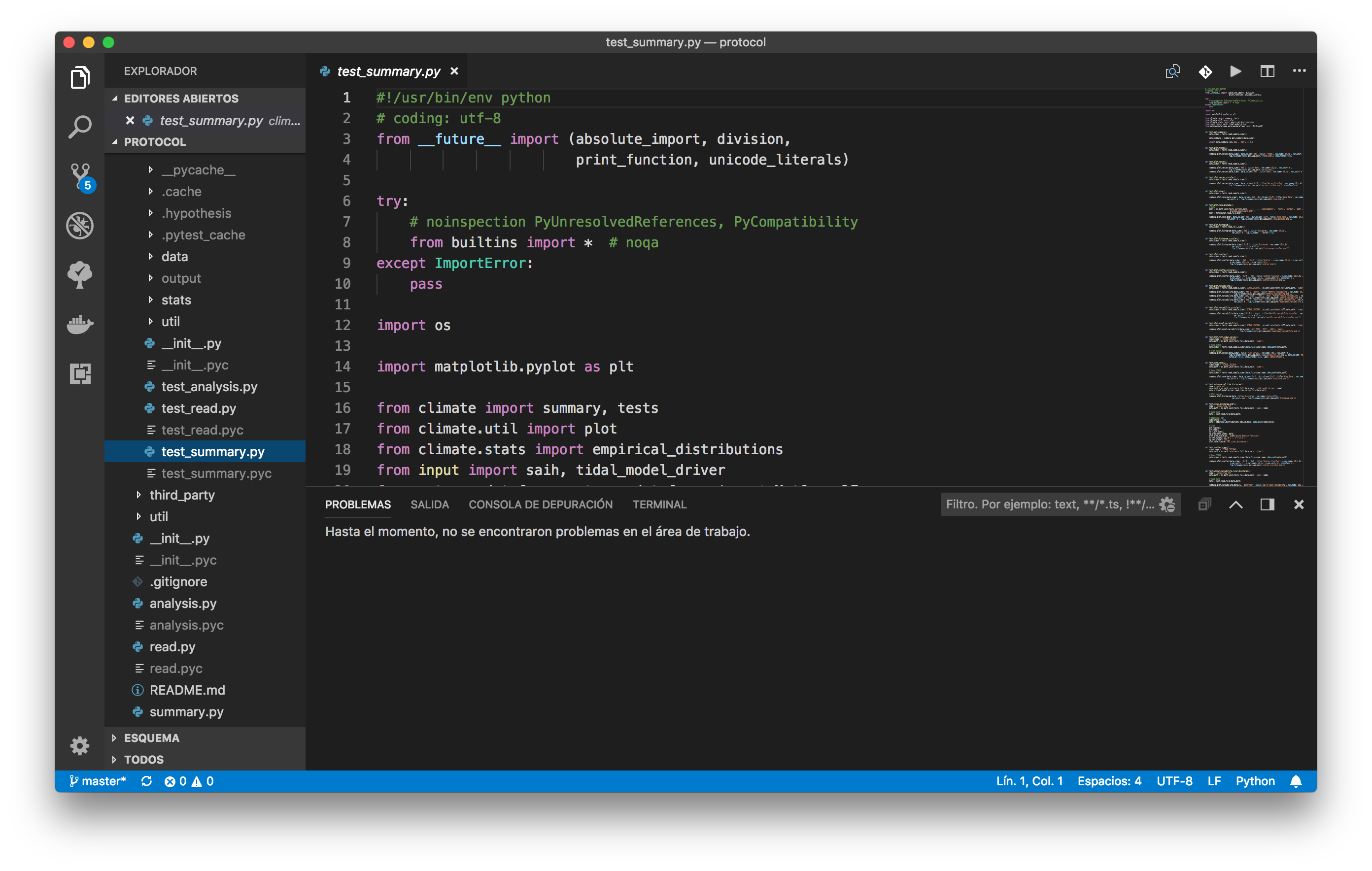
Visual Studio Code
PyCharm (need to be installed separately from Anaconda)
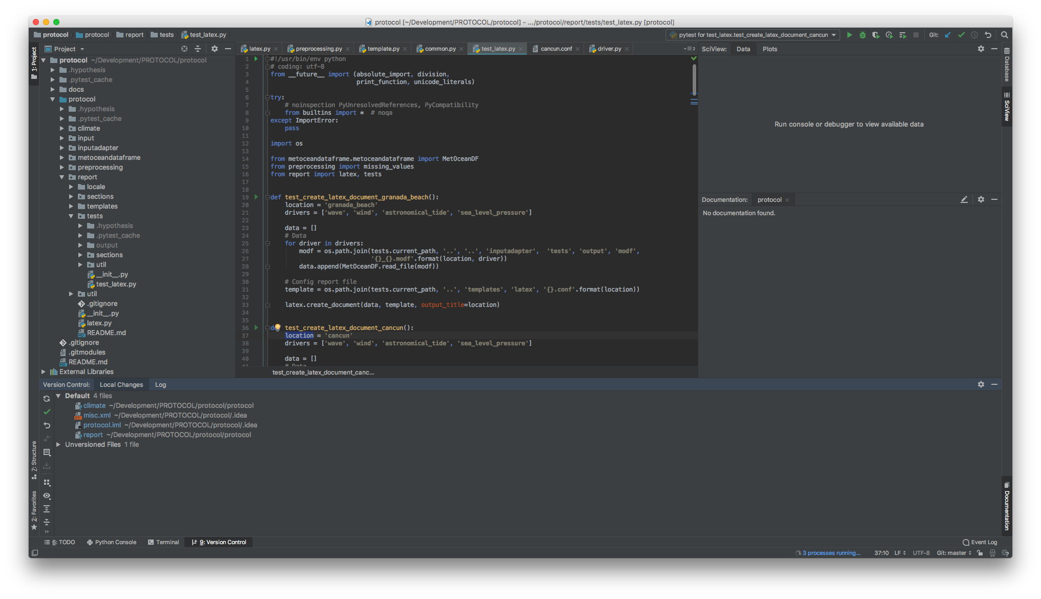
| Editor | Learning curve | Users | Benefits |
|---|---|---|---|
| Spyder | pretty short | Matlab and R background | mature, many features |
| Jupyter | smooth | teachers | interactive |
| Visual Studio Code | moderate | scientifics / developers | code quality |
| PyCharm | steep | developers | professional code |
Bibliography
- A Whirlwind Tour of Python by Jake VanderPlas (2016). ISBN: 9781492037859 (pdf version)
- Python for Data Analysis (2nd Edition) by Wes McKinney (2017). ISBN: 1491957662.
- Pandas Cookbook: Recipes for Scientific Computing, Time Series Analysis and Data Visualization using Python by Theodore Petrou (2017). ISBN: 9781784393878.
MOOC (Online Courses)
Basic Python: Operators
| Operator | Name | Description |
|---|---|---|
a + b |
Addition | Sum of a and b |
a - b |
Subtraction | Difference of a and b |
a * b |
Multiplication | Product of a and b |
a / b |
True division | Quotient of a and b |
a // b |
Floor division | Quotient of a and b, removing fractional parts |
a % b |
Modulus | Integer remainder after division of a by b |
a ** b |
Exponentiation | a raised to the power of b |
-a |
Negation | The negative of a |
+a |
Unary plus | a unchanged (rarely used) |
# addition, subtraction, multiplication
print((4 + 8) * (6.5 - 3))
42.0
# Division
print(11 / 2)
5.5
Assignment Operations
a = 24
print(a)
24
a = a + 2
print(a)
26
print(a + 2)
28
a += 2  # equivalent to a = a + 2
print(a)
28
Comparison Operations
| Operation | Description |
|---|---|
a == b |
a equal to b |
a < b |
a less than b |
a <= b |
a less than or equal to b |
a != b |
a not equal to b |
a > b |
a greater than b |
a >= b |
a greater than or equal to b |
print(22 / 2 == 10 + 1)
True
# 25 is even
print(25 % 2 == 0)
False
# 66 is odd
print(66 % 2 == 0)
True
# check if a is between 15 and 30
a = 25
print(15 < a < 30)
True
Boolean Operations
x = 4
print((x < 6) and (x > 2))
True
print((x > 10) or (x % 2 == 0))
True
print(not (x < 6))
False
Membership Operators
| Operator | Description |
|---|---|
a in b |
True if a is a member of b |
a not in b |
True if a is not a member of b |
print(1 in [1, 2, 3])
True
print(2 not in [1, 2, 3])
False
Built-In Types
| Type | Example | Description |
|---|---|---|
int |
x = 1 |
integers (i.e., whole numbers) |
float |
x = 1.0 |
floating-point numbers (i.e., real numbers) |
complex |
x = 1 + 2j |
Complex numbers (i.e., numbers with real and imaginary part) |
bool |
x = True |
Boolean: True/False values |
str |
x = 'abc' |
String: characters or text |
NoneType |
x = None |
Special object indicating nulls |
Integers
5 / 2
2.5
# Floor division
5 // 2
2
Floating-Point Numbers
x = 0.000005
y = 5e-6
print(x == y)
True
print(0.1 + 0.2 == 0.3)
False
Floating-point precision is limited, which can cause equality tests to be unstable
String Type
message = "what do you like?"
print(message)
what do you like?
response = "spam"
print(response)
spam
# length of string
print(len(response))
4
# Make upper-case. See also str.lower()
print(response.upper())
SPAM
# Capitalize. See also str.title()
print(message.capitalize())
What do you like?
# concatenation with +
print(message + response)
what do you like?spam
# multiplication is multiple concatenation
print(5 * response)
spamspamspamspamspam
# Access individual characters (zero-based indexing)
print(message[0])
w
# index range is checked
print(message[59])
---------------------------------------------------------------------------
IndexError                                Traceback (most recent call last)
<ipython-input-46-ecd28c2b2692> in <module>
      1 # index range is checked
----> 2 print(message[59])

IndexError: string index out of range
Boolean Type
result = 4 < 5
print(result)
True
TrueandFalsemust be capitalized!
Exercises
- How many hours are in a year?
- How many minutes are in a decade?
- How many seconds old are you?
Leap years can be ignored
# How many hours are in a year?
print(24 * 365)
8760
# How many minutes are in a decade?
print(60 * 24 * (365 * 10))
5256000
# How many seconds old are you?
print(60 * 60 * 24 * (365 * 23))
725328000
Built-In Data Structures
| Type Name | Example | Description |
|---|---|---|
list |
[1, 2, 3] |
Ordered collection |
tuple |
(1, 2, 3) |
Immutable ordered collection |
dict |
{'a': 1, 'b': 2, 'c': 3} |
Unordered (key,value) mapping (ordered in Python 3.7+) |
set |
{1, 2, 3} |
Unordered collection of unique values |
Lists
lst = [2, 3, 5, 7]
# Length of a list
print(len(lst))
4
# Append a value to the end
lst.append(11)
print(l)
---------------------------------------------------------------------------
NameError                                 Traceback (most recent call last)
<ipython-input-56-fb7dd1e7c8da> in <module>
      1 # Append a value to the end
      2 lst.append(11)
----> 3 print(l)

NameError: name 'l' is not defined
# Addition concatenates lists
print(lst + [13, 17, 19])
[2, 3, 5, 7, 11, 13, 17, 19]
# sort() method sorts in-place
lst = [2, 5, 1, 6, 3, 4]
lst.sort()
print(lst)
[1, 2, 3, 4, 5, 6]
lst = [1, "two", 3.14, [0, 3, 5]]
print(lst)
[1, 'two', 3.14, [0, 3, 5]]
List indexing and slicing
lst = [2, 3, 5, 7, 11]
print(lst[0])
2
print(lst[1])
3
print(lst[-1])
11
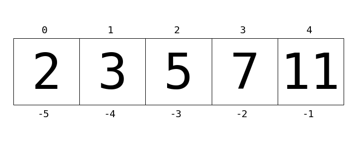
print(lst[0:3])
[2, 3, 5]
print(lst[:3])
[2, 3, 5]
print(lst[::2]) # equivalent to l[0:len(l):2]
[2, 5, 11]
lst[0] = 100
print(lst)
[100, 3, 5, 7, 11]
Dictionaries
numbers = {"one": 1, "two": 2, "three": 3}
# Access a value via the key
print(numbers["two"])
2
# Set a new key:value pair
numbers["ninety"] = 90
print(numbers)
{'one': 1, 'two': 2, 'three': 3, 'ninety': 90}
Exercises
- Create a dictionary with the following birthday information:
- Albert Einstein - 03/14/1879
- Benjamin Franklin - 01/17/1706
- Ada Lovelace - 12/10/1815
- Donald Trump - 06/14/1946
- Rowan Atkinson - 01/6/1955
- Check if Donald Trump is in our dictonary
- Get Albert Einstein's birthday
# Create a dictionary with the following birthday information
birthdays = {
    "Albert Einstein": "03/14/1879",
    "Benjamin Franklin": "01/17/1706",
    "Ada Lovelace": "12/10/1815",
    "Donald Trump": "06/14/1946",
    "Rowan Atkinson": "01/6/1955",
}
# Check if Donald Trump is in our dictonary
print("Donald Trump" in birthdays)
True
# Get Albert Einstein's birthday
print(birthdays["Albert Einstein"])
03/14/1879
Control Flow
Conditional Statements: if-elif-else
x = 15

if x == 0:
    print(x, "is zero")
elif (x > 0) and (x < 10):
    print(x, "is between 0 and 10")
elif (x > 10) and (x < 20):
    print(x, "is between 10 and 20")
else:
    print(x, "is negative")
print("hola mundo")
15 is between 10 and 20
hola mundo
Loops: for
n = [2, 3, 5, 7]
for e in n:
    print(e)
2
3
5
7
Please avoid Matlab-like for statements with range
for e in range(len(n)):
    print(n[e])
2
3
5
7
m = range(5)  # m = [0, 1, 2, 3, 4]
for _ in m:
    print("hola")
hola
hola
hola
hola
hola
for index, value in enumerate(n):
    print("The value of index ", index, " is ", value)
The value of index  0  is  2
The value of index  1  is  3
The value of index  2  is  5
The value of index  3  is  7
Loops: while
i = 0
while i < 10:
    print(i)
    i += 1
0
1
2
3
4
5
6
7
8
9
Be careful with while loops
Functions
Defining Functions
import time


def cabecera():
    mensaje = "Este programa está escrito por Roberto Gómez"
    mensaje += ". Copyright " + time.strftime("%d-%m-%Y")

    return mensaje


print(cabecera())
Este programa está escrito por Roberto Gómez. Copyright 29-10-2019
def cabecera_mejorada(autor):
    mensaje = "Este programa está escrito por "
    mensaje += autor
    mensaje += ". Copyright " + time.strftime("%d-%m-%Y")

    return mensaje


print(cabecera_mejorada("Roberto Gómez"))
Este programa está escrito por Roberto Gómez. Copyright 29-10-2019
print(cabecera_mejorada("Alfonso Hernández"))
Este programa está escrito por Alfonso Hernández. Copyright 29-10-2019
def fibonacci(n):
    l = []
    a = 0
    b = 1
    while len(l) < n:
        l.append(a)
        c = a + b
        a = b
        b = c
    return l
print(fibonacci(10))
[0, 1, 1, 2, 3, 5, 8, 13, 21, 34]
print(fibonacci(3))
[0, 1, 1]
Default Argument Values
def fibonacci(n, start=0):
    fib = []
    a = 0
    b = 1
    while len(fib) < n:
        if a >= start:
            fib.append(a)
        c = a + b
        a = b
        b = c
    return fib
print(fibonacci(10))
[0, 1, 1, 2, 3, 5, 8, 13, 21, 34]
print(fibonacci(10, 5))
[5, 8, 13, 21, 34, 55, 89, 144, 233, 377]
## Keyword arguments
print(fibonacci(start=5, n=10))
[5, 8, 13, 21, 34, 55, 89, 144, 233, 377]
from datetime import datetime, timedelta

dt1 = datetime(2005, 7, 14, 12, 30)

dt2 = dt1 + timedelta(hours=5)

print(dt2)
2005-07-14 17:30:00
timedelta([days[, seconds[, microseconds[, milliseconds[, minutes[, hours[, weeks]]]]]]])
All arguments are optional and default to 0. Arguments may be ints, longs, or floats, and may be positive or negative.
Documentation strings (docstrings)
- Python documentation strings (docstrings) provide a convenient way of associating documentation with Python functions and modules.
- Docstrings can be written following several styles. We use Google Python Style Guide.
- An object's docsting is defined by including a string constant as the first statement in the function's definition.
- Unlike conventional source code comments the docstring should describe what the function does, not how.
- All functions should have a docstring.
- This allows to inspect these comments at run time, for instance as an interactive help system, or export them as HTML, LaTeX, PDF or other formats.
def fibonacci(n, start=0):
    """Build a Fibonacci series with n elements starting at start

    Args:
        n: number of elements
        start: lower limit. Default 0

    Returns:
        A list with a Fibonacci series with n elements
    """
    fib = []
    a = 0
    b = 1
    while len(fib) < n:
        if a >= start:
            fib.append(a)
        c = a + b
        a = b
        b = c
    return fib
Exercises
- Reverse a string
Example input: "cool" output: "looc"
- Calculate the Hamming difference between two DNA strands
A mutation is simply a mistake that occurs during the creation or copying of a nucleic acid, in particular DNA. By counting the number of differences between two homologous DNA strands taken from different genomes with a common ancestor, we get a measure of the minimum number of point mutations that could have occurred on the evolutionary path between the two strands.
Example:
GAGCCTACTAACGGGAT
CATCGTAATGACGGCCT
^ ^ ^ ^ ^ ^^
Given a number, determine if it is prime
Given a number, determine what the nth prime is
# Reverse a string
cadena1 = "cool"
cadena2 = ""
for c in cadena1[-1::-1]:
    cadena2 = cadena2 + c
print(cadena2)
looc
cadena1 = "hola mundo"
cadena2 = ""
for c in cadena1[-1::-1]:
    cadena2 = cadena2 + c
print(cadena2)
odnum aloh
cadena = "cool"


def invertir_cadena(cadena_entrada):
    cadena_salida = ""
    for c in cadena_entrada[-1::-1]:
        cadena_salida += c
    return cadena_salida


print(invertir_cadena(cadena))
looc
print(invertir_cadena("Hola mundo"))
odnum aloH
# Hamming distance
c1 = "GAGCCTACTAACGGGAT"
c2 = "CATCGTAATGACGGCCT"


def hamming(dna_1, dna_2):
    l = len(dna_1)
    hamming = 0
    for i in range(l):
        if dna_1[i] != dna_2[i]:
            hamming += 1
    return hamming


print(hamming(c1, c2))
7
print(hamming("TAGAG", "TAGAA"))
1
# Prime number
number = 4


def is_prime(number):
    is_prime = True
    for x in range(2, number):
        if (number % x) == 0:
            is_prime = False
    return is_prime


is_prime(number)
False
# Nth Prime
def n_prime(nth):
    n = 2
    primes = []
    while len(primes) < nth:
        if is_prime(n):
            primes.append(n)
        n += 1
    return primes[-1]


print(n_prime(6))
13
print(n_prime(1))
2
Modules and Packages
Loading Modules: the import Statement
Explicit module import
External file required:
import functions  # without .py extension

print(functions.fibonacci(5))
[0, 1, 1, 2, 3]
Explicit module import by alias
import functions as f

print(f.fibonacci(5))
[0, 1, 1, 2, 3]
Explicit import of module contents
from functions import fibonacci

print(fibonacci(5))
[0, 1, 1, 2, 3]
Importing from Third-Party Modules
The best way to import libraries is included in their official help
import math
import numpy as np
from scipy import linalg, optimize
import pandas as pd
import matplotlib as mpl
import matplotlib.pyplot as plt
import sympy
Code Style
- Style Guide for Python Code: PEP8.
- Use only English (ASCII) characters for variables, functions and files.
- Name your variables, functions and files consistently: the convention is to use lower_case_with_underscores.
- We all use double-quoted strings to be consistent. Nevertheless, single-quoted strings and double-quoted strings are the same. PEP does not make a recommendation for this, except for function documentation where tripe-quote strings should be used.
PEP8 exceptions
- Long lines
It is very conservative and requires limiting lines to 79 characters. We use all lines to a maximum of 88 characters. This is the default behaviour in The Black code style.
- Disable checks in one line
Skip validation in one line by adding following comment:
# nopep8
Data Science Tools
NumPy: Numerical Python
import numpy as np

x = np.arange(1, 10)
print(x)
[1 2 3 4 5 6 7 8 9]
print(x ** 2)
[ 1 4 9 16 25 36 49 64 81]
y = x.reshape((3, 3))
print(y)
[[1 2 3]
 [4 5 6]
 [7 8 9]]
print(y.T)
[[1 4 7]
 [2 5 8]
 [3 6 9]]
a = np.array([[1, 0], [0, 1]])
b = np.array([[4, 1], [2, 2]])

print(np.dot(a, b))
[[4 1]
 [2 2]]
Vectorization
Arrays enable you to express batch operations on data without writing any for loops. This is usually called vectorization:
- vectorized code is more concise and easier to read
- fewer lines of code generally means fewer bugs
- the code more closely resembles standard mathematical notation
But:
sometimes it's difficult to move away from the for-loop school of thought
Pandas: Labeled Column-oriented Data
- fast and efficient Series (1-dimensional) and DataFrame (2-dimensional) heterogeneous objects for data manipulation with integrated indexing
- tools for reading and writing data from different formats: CSV and text files, Microsoft Excel, SQL databases, HDF5...
- intelligent label-based slicing
- time series-functionality
- integrated handling of missing data
import pandas as pd

df = pd.DataFrame(
    {"label": ["A", "B", "C", "A", "B", "C"], "value": [1, 2, 3, 4, 5, 6]}
)
print(df)

df.to_excel("file.xlsx")
  label  value
0     A      1
1     B      2
2     C      3
3     A      4
4     B      5
5     C      6
print(df["label"])
0    A
1    B
2    C
3    A
4    B
5    C
Name: label, dtype: object
print(df["value"].sum())
21
print(df.groupby("label").sum())
       value
label
A          5
B          7
C          9
Exercises
External files required:
Matplotlib scientific visualization
import matplotlib.pyplot as plt
x = np.linspace(0, 10)  # range of values from 0 to 10
y = np.sin(x)  # sine of these values
plt.plot(x, y)
# plot as a line
[<matplotlib.lines.Line2D at 0x12ac5fa58>]
SciPy: Scientific Python
scipy.fftpack: Fast Fourier transformsscipy.integrate: Numerical integrationscipy.interpolate: Numerical interpolationscipy.linalg: Linear algebra routinesscipy.optimize: Numerical optimization of functionsscipy.sparse: Sparse matrix storage and linear algebrascipy.stats: Statistical analysis routines
Sympy: Symbolic Python
from IPython.display import display
from sympy import symbols

# Pretty printing
from sympy import init_printing

init_printing()

x, y = symbols("x y")
expr = x + 2 * y

display(expr)
Derivative of $$sin(x)e^x$$
from sympy import diff, sin, exp, pprint

out = diff(sin(x) * exp(x), x)

display(out)
Compute $$\int(e^x\sin{(x)} + e^x\cos{(x)})\,dx$$
from sympy import integrate, cos

out = integrate(exp(x) * sin(x) + exp(x) * cos(x), x)

display(out)
